Calculus I: Appendix-E: Derivation of the dot product and the projection vectors

1) The dot product:

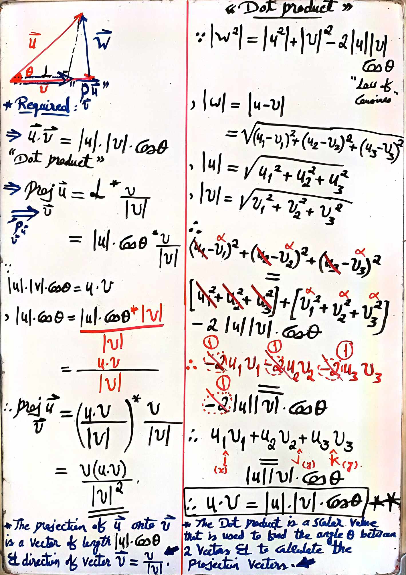
• Recall, 2 intersecting vectors $u$ and $v$ together with the resultant vetcor $w$; such that, \(w = u - v\)

• From the “Law of Cosines”:

\[Since, ||w||^2 = ||u||^2 + ||v||^2 - 2 * ||u||^2 * ||v||^2 * cos(\theta)\] \[Then, cos(\theta) = (||w||^2 - ||u||^2 - ||v||^2) / -2 * ||u||^2 * ||v||^2\ Lemma\.01\] \[-------\] \[Since, ||w|| = \sqrt{(u_x - v_x)^2 + (u_y - v_y)^2 + (u_z - v_z)^2}\] \[||v|| = \sqrt{\{v_x}^2 + {v_y}^2 + {v_z}^2\}\] \[||u|| = \sqrt{\{u_x}^2 + {u_y}^2 + {u_z}^2\}\] \[||w|| = ||u-v|| = \sqrt{\{(u_x - v_x)}^2 + {(u_y - v_y)}^2 + {(u_z - v_z)}^2\}\] \[Then,\ Lemma.02:\] \[1)\ ||v||^2 = {v_x}^2 + {v_y}^2 + {v_z}^2\] \[2)\ ||u||^2 = {u_x}^2 + {u_y}^2 + {u_z}^2\] \[3)\ ||w||^2 = {u_x - v_x}^2 + {u_y - v_y}^2 + {u_z - v_z}^2\] \[= ({u_x}^2 -2{u_x}{v_x} + {v_x}^2) + ({u_y}^2 -2{u_y}{v_y} + {v_y}^2) + ({u_z}^2 -2{u_z}{v_z} + {v_z}^2)\] \[= ||u||^2 + ||v||^2 -2({u_x}{v_x} + {u_y}{v_y} + {u_z}{v_z})\] \[-------\]

• By back-substitution in $Lemma.01$:

\[cos(\theta) = (||w||^2 - ||u||^2 - ||v||^2) / -2 * ||u||^2 * ||v||^2 = {(R.H.S)}_1 / {(R.H.S)}_2\] \[{(R.H.S)}_1 = (||w||^2 - ||u||^2 - ||v||^2)\] \[= -2({u_x}{v_x} + {u_y}{v_y} + {u_z}{v_z})\] \[{(R.H.S)}_2 = -2 * ||u||^2 * ||v||^2\] \[Hence, cos(\theta) = {(R.H.S)}_1 / {(R.H.S)}_2\] \[= -2({u_x}{v_x} + {u_y}{v_y} + {u_z}{v_z}) / -2 * ||u||^2 * ||v||^2\] \[= ({u_x}{v_x} + {u_y}{v_y} + {u_z}{v_z}) / ||u||^2 * ||v||^2\]

• And, by definition $({u_x}{v_x} + {u_y}{v_y} + {u_z}{v_z})$ yields $u.v$, the dot product or the inner product.

\[Thence, cos(\theta) = u.v / ||u|| * ||v||\] \[And, u.v = ||u|| * ||v|| * cos(\theta)\]

2) Projection vectors:

• Definition: The projection vector $\vec{proj_{\vec{v}}} \vec{u}$ of a vector $\vec{u}$, is the vector component of that vector, that is coincident to the projectile vector $\vec{v}$, multiplied by the unit vector of the projectile vector (i.e., the direction).

• For a productive proof, let vector $\vec{u}$ be our target vector, the one we would like to find its vector components in the direction of another contigous vectors, and vector $\vec{v}$ be the projectile (aka. base) vector the one we would like to utilize its direction to find the projection vector.

1) Finding the norm of the vector component $

\vec{u_x}

$ that is coincident to the projectile vector $\vec{v}$:

\[Since,cos(\theta)=||\vec{u_x}||/||\vec{u}||\] \[Then,||\vec{u_x}||=||\vec{u}||*cos(\theta)\]

2) Finding the vector norm $

\vec{v}

$ of the projectile vector $\vec{v}$:

\[||\vec{v}||=\sqrt{\{v_x}^2+{v_y}^2+{v_z}^2\}\]

3) Finding the normalization ratio using the scalar division property $\vec{v_{unit}}=\vec{v}/

\vec{v}

$ of the projectile vector (base vector).

4) Using the scalar multiplication property $

\vec{u_x}

*\vec{v_{unit}}$:

$Lemma.01$

\[||\vec{u_x}||*\vec{v_{unit}}=(||\vec{u}||*cos(\theta))\*\vec{v_{unit}}\] \[Since,\vec{u}.\vec{v}=||\vec{u}||*||\vec{v}||\*cos(\theta)\]

$Lemma.02$

\[Then,||\vec{u}||*cos(\theta)=(\vec{u}.\vec{v})/||\vec{v}||\]

5) Then, from $Lemma.01$ and $Lemma.02$, we can deduce the projection vector formula in terms of the dot product between 2 vectors as follows:

\[\vec{proj_{\vec{v}}}\vec{u}=[({\vec{u}}.{\vec{v}})*{\vec{v_{unit}}}]/||\vec{v}||\]

6) Another formula when $\vec{v_{unit}}$ is broken:

\[\vec{proj_{\vec{v}}}\vec{u}=[\vec{u}.\vec{v}*\vec{v}]/||\vec{v}||^2\]

Note:

• This is could be applied to other components of vector $\vec{u}$, the $\vec{u_y}$, and the $\vec{u_z}$, and any vector could be utilized as the base or the projectile vector.
• The projection vector of vector $\vec{u}$ on itself $\vec{proj_{\vec{u}}} \vec{u}$ is the vector $\vec{u}$ itself scaled with the length of one of its vector components.

3) Usages Review:

1) Finding the work done by a force vector $(F)$ to move an object a displacement $(D)$ with an inscribed angle $(a)$, formula (Physics):

\[W = F.D = ||F|| * ||D|| * cos(a) = \sum_{i=0}^{n} u_i v_i = u_0 v_0+u_1 v_1+u_2 v_2+...+ u_{n-1} v_{n-1} + u_n v_n\]

2) Finding the inscribed angle (<a) between 2 intersecting vectors, formula:

\[m(a) = acos(u.v/(||u|| * ||v||))\]

where u.v can be evaluated using the Riemann’s sum formula (Trigo./Physics).

3) Finding whether 2 intersecting vectors are orthogonal, formula: $u.v =

u

*

v

* cos(PI/2) = ZERO.$ (Geometry).

4) Finding projection vectors, formula: “the vector projection of $u$ onto $v$”, formula:

\[proj_{v}^{u} = (||u|| * cos(a)) * (v/||v||) = (u.v / ||v||^2) * v\]

where $(

u

* cos(a))$ is the length of the triangle base, and $(v/

v

)$ is the unit vector form (normalized) of $v$.

5) Finding the total electromotive force (EMF) in a closed circuit loop, formula (aka. Ohm’s Law):

\[V = I * R * cos(0)\]

6) Finding the driving arterial blood pressure in a closed arterial circuitry, formula (Hemodynamics):

\[BP = CO * SVR * cos(0)\]

References:

• Thomas’ Calculus $14^{th}e$: Ch.12 Vectors & Geometry of Space: Section.12.3. (The Dot Product).
• Guyton and Hall Textbook of Medical Physiology $13^{th}e$
• Applied Linear Algebra $2^{nd}e$ Springer